Diffuse Materials

Created

2021/03/26

1. A Simple Diffuse Material

난반사가 되는 Object는 빛을 발산하지 않기 때문에 Object 자체가 갖고 있는 본연의 색을 통해 단순히 주변 환경의 색을 적절히 조절하여 취하게 된다.

난반사 Object들은 정반사를 하지 않기 때문에 흡수하는 성질을 갖고 있다. 특히 표면이 어두울수록 흡수를 잘하게 된다. 이러한 특성을 살리기 앞서서 가장 먼저 난반사를 구현해줘야 한다. 난반사는 무작위한 방향을 만들어주는 알고리즘을 이용하여 비슷하게 만들 수 있으며 이를 통해 Object의 표면을 녹슨 질감을 줄 수 있다. 이 방법이 난반사 표면을 가장 이상적으로 표현할 수 있는 가장 쉬운 방법이다. 무작위한 방향을 만들어주는 방법에 대해 알아보자.

점

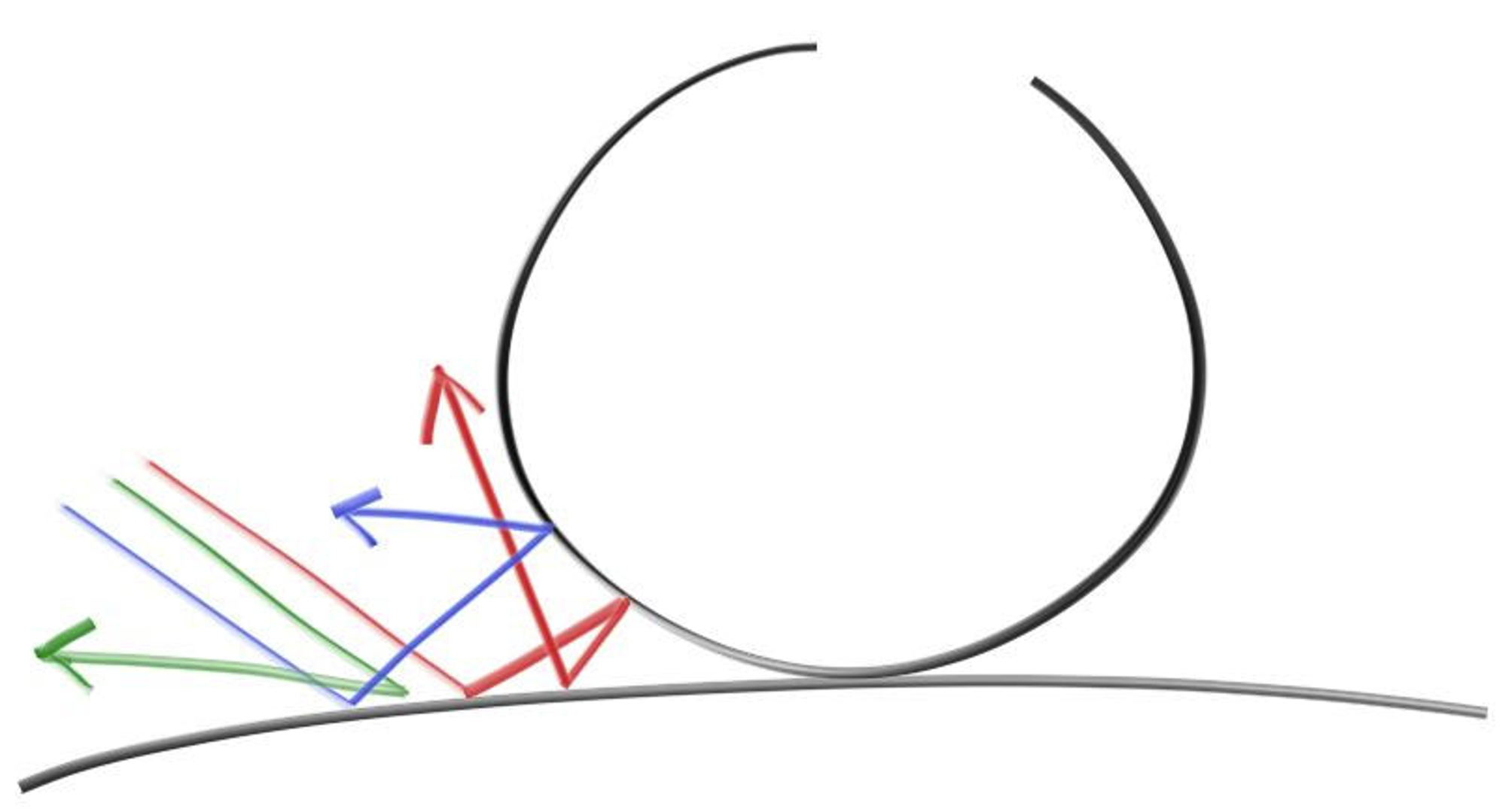
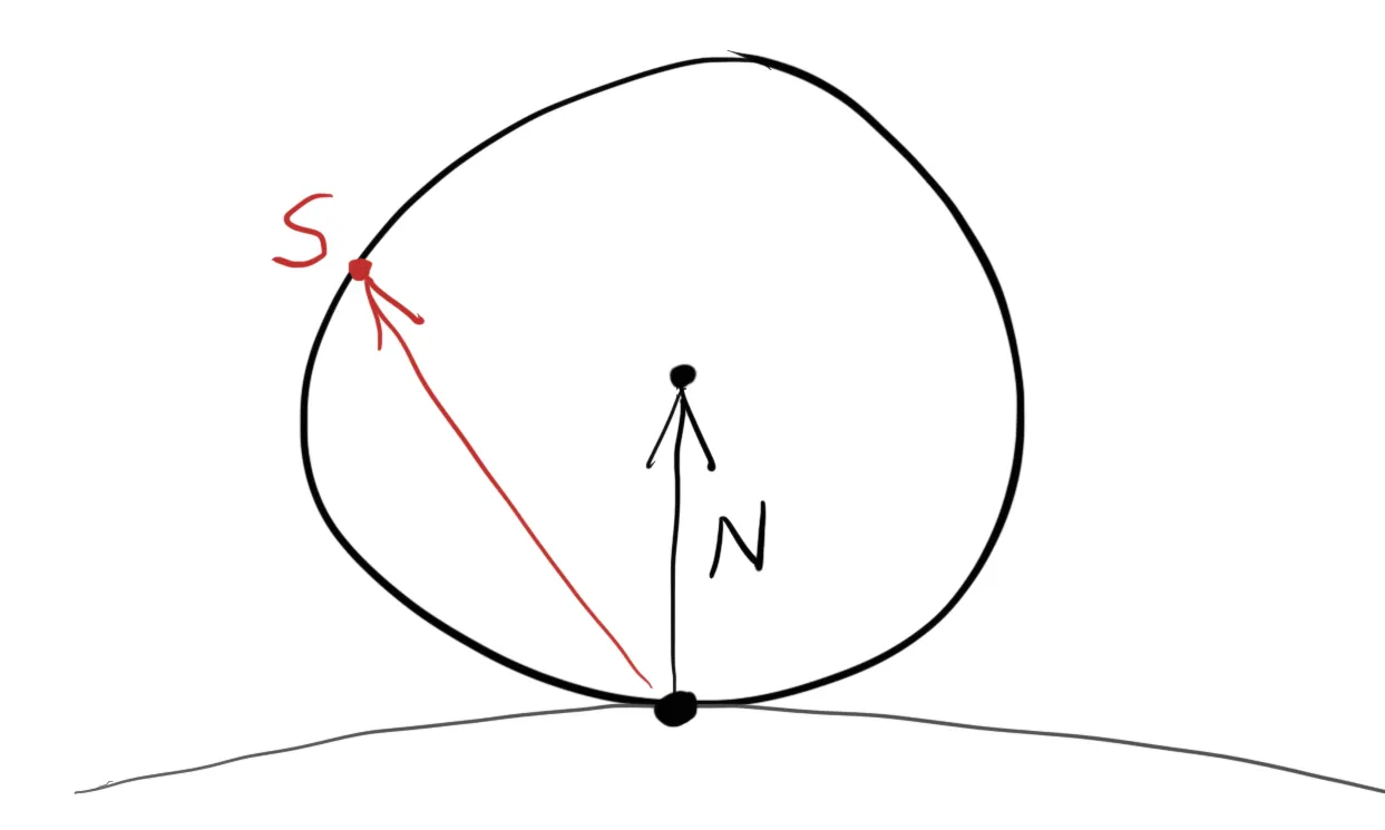
P

에서 단위 구 2개가 접하고 있다고 해보자. 이에 따라 접하는 면에 대한 단위 Normal을

n

이라 했을 때 구체들의 중심점은

P+n

P-n

이 된다. 중심점이

P-n

인 구체는 표면 안쪽이라고 보면 되고, 중심점이

P+n

인 구체는 표면 바깥쪽이라고 보면 된다. 접하고 있는 구체 중에 중심점이

P+n

인 바깥쪽 구체에서 내부의 무작위한 점을

S

라고 해보자. ray가 접점인

P

를 향해 온다고 할 때, 이를 그대로 무작위 점

S

로 보내버리면 무작위한 방향을 생성해낼 수 있다. 무작위하게 생성된 방향을 Vector로 나타내면

S-P

가 된다. (이는 곧 점

P

P -n

을 중심으로 갖는 구체의 Normal + 점

S

로 나타낼 수 있다. 눈치가 좋은 사람이라면, 이 방법이 곧 Normal에 의존적인 것을 알 수 있을 것이다.)

중심점

P-n

으로 예시로 든 Object가 World의 Object이고, 중심점

P+n

으로 예시를 든 Object가 무작위 방향 생성을 위한 가상의 Object라고 생각하면 되겠다.

방법은 위와 같으니, 단위 구체 내부의 무작위 점을 잡아만 주면 된다. 이에 대해 가장 쉬운 알고리즘은 Rejection이다. 범위가

-1

에서

1

사이에 있는

x

y

z

를 무작위로 정하여 한 점을 생성하고, 만일 이 점을 구체에 적용했을 때 구체 밖이 되면 무작위로 잡았던 점을 Reject하고 다시 임의의 점을 잡아 반복한다. vec3.h 내부에 아래와 같이 random 함수와 random 함수를 통해 반환 받은 점을 구체 내의 점인지 확인하여 사용할 수 있게 해주는 random_in_unit_sphere라는 함수를 추가한다.

#ifndef VEC3_H
# define VEC3_H

# include "rtweekend.h"
# include <cmath>
# include <iostream>

using std::sqrt;

class vec3
{
    public:
        vec3() : e{0,0,0} {}
        vec3(double e0, double e1, double e2) : e{e0, e1, e2} {}

        double x() const { return e[0]; }
        double y() const { return e[1]; }
        double z() const { return e[2]; }

        vec3 operator-() const { return vec3(-e[0], -e[1], -e[2]); }
        double operator[](int i) const { return e[i]; }
        double& operator[](int i) { return e[i]; }

        vec3& operator+=(const vec3 &v)
				{
            e[0] += v.e[0];
            e[1] += v.e[1];
            e[2] += v.e[2];
            return *this;
        }

        vec3& operator*=(const double t)
				{
            e[0] *= t;
            e[1] *= t;
            e[2] *= t;
            return *this;
        }

        vec3& operator/=(const double t)
				{
            return *this *= 1/t;
        }

        double length() const
				{
            return sqrt(length_squared());
        }

        double length_squared() const
				{
            return e[0]*e[0] + e[1]*e[1] + e[2]*e[2];
        }

				inline static vec3 random()
				{
					return (vec3(random_double(), random_double(), random_double()));
				}

				inline static vec3 random(double min, double max)
				{
					return (vec3(random_double(min, max), random_double(min, max), random_double(min, max)));
				}


    public:
        double e[3];
};

// Type aliases for vec3
using point3 = vec3;   // 3D point
using color = vec3;    // RGB color

// vec3 Utility Functions
inline std::ostream& operator<<(std::ostream &out, const vec3 &v)
{
    return out << v.e[0] << ' ' << v.e[1] << ' ' << v.e[2];
}

inline vec3 operator+(const vec3 &u, const vec3 &v)
{
    return vec3(u.e[0] + v.e[0], u.e[1] + v.e[1], u.e[2] + v.e[2]);
}

inline vec3 operator-(const vec3 &u, const vec3 &v)
{
    return vec3(u.e[0] - v.e[0], u.e[1] - v.e[1], u.e[2] - v.e[2]);
}

inline vec3 operator*(const vec3 &u, const vec3 &v)
{
    return vec3(u.e[0] * v.e[0], u.e[1] * v.e[1], u.e[2] * v.e[2]);
}

inline vec3 operator*(double t, const vec3 &v)
{
    return vec3(t*v.e[0], t*v.e[1], t*v.e[2]);
}

inline vec3 operator*(const vec3 &v, double t)
{
    return t * v;
}

inline vec3 operator/(vec3 v, double t)
{
    return (1/t) * v;
}

inline double dot(const vec3 &u, const vec3 &v)
{
    return u.e[0] * v.e[0]
         + u.e[1] * v.e[1]
         + u.e[2] * v.e[2];
}

inline vec3 cross(const vec3 &u, const vec3 &v)
{
    return vec3(u.e[1] * v.e[2] - u.e[2] * v.e[1],
                u.e[2] * v.e[0] - u.e[0] * v.e[2],
                u.e[0] * v.e[1] - u.e[1] * v.e[0]);
}

inline vec3 unit_vector(vec3 v)
{
    return v / v.length();
}

vec3 random_in_unit_sphere()
{
	while (true)
	{
		auto p = vec3::random(-1, 1);
		if (p.length_squared() >= 1)
			continue;
		return (p);
	}
}

#endif
C++
복사

이처럼 무작위 방향을 생성할 수 있게 되었다면, 각 Pixel마다 색상을 결정하는 ray_color 함수에서 이 무작위 방향을 이용할 수 있도록 main.cpp 역시 아래처럼 수정한다.

#include "rtweekend.h"
#include "color.h"
#include "hittable_list.h"
#include "sphere.h"
#include "camera.h"
#include <iostream>

color ray_color(const ray& r, const hittable& world)
{
	hit_record rec;
	if (world.hit(r, 0, infinity, rec))
	{
		point3 target = rec.p + rec.normal + random_in_unit_sphere();
		return (0.5 * ray_color(ray(rec.p, target - rec.p), world));
	}
	vec3 unit_direction = unit_vector(r.direction());
	auto t = 0.5 * (unit_direction.y() + 1.0);
	return (1.0 - t) * color(1.0, 1.0, 1.0) + t * color(0.5, 0.7, 1.0);
}

int main(void)
{
	// Image
	const auto aspect_ratio = 16.0 / 9.0;
	const int image_width = 400;
	const int image_height = static_cast<int>(image_width / aspect_ratio);
	const int samples_per_pixel = 100;

	// World
	hittable_list world;
	world.add(make_shared<sphere>(point3(0, 0, -1), 0.5));
	world.add(make_shared<sphere>(point3(0, -100.5, -1), 100));

	// Camera
	camera cam;

	// Render
	std::cout << "P3\n" << image_width << ' ' << image_height << "\n255\n";

	for (int j = image_height - 1; j >= 0; --j)
	{
		std::cerr << "\rScanlines Remaining: " << j << ' ' << std::flush;
		for (int i = 0; i < image_width; ++i)
		{
			color pixel_color(0, 0, 0);
			for (int s = 0; s < samples_per_pixel; ++s)
			{
				auto u = (i + random_double()) / (image_width - 1);
				auto v = (j + random_double()) / (image_height - 1);
				ray r = cam.get_ray(u, v);
				pixel_color += ray_color(r, world);
			}
			write_color(std::cout, pixel_color, samples_per_pixel);
		}
	}

	std::cerr << "\nDone.\n";

	return (0);
}
C++
복사

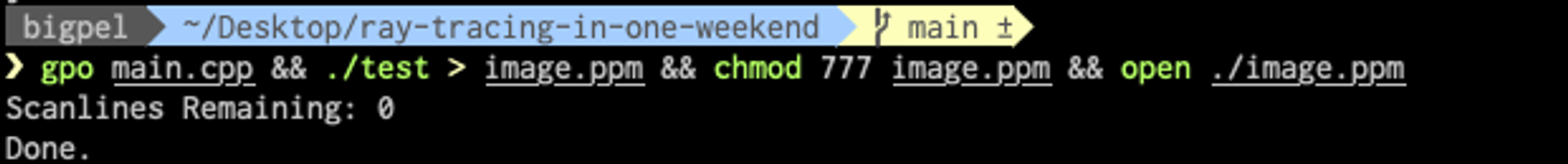
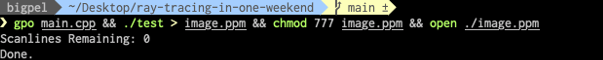
난반사 구현을 위해 무작위 방향을 생성한 Vector가 target이 되는데, 이것이 곧 반사된 빛이기 때문에 ray 객체를 생성하여 재귀적으로 ray_color를 호출하도록 만든다. 이렇게 재귀적으로 ray_color를 호출하는 것을 생각해보면, 끊임 없이 함수를 호출하게 되기 때문에 얼만큼의 Child를 둘 것인지 정하는 것이 중요하다. 그렇지 않으면 끊임 없는 호출에 Stack이 꽉차 터지게 되어 아래 사진과 같이 오류를 볼 수 있다.

2. Limiting the Number of Child Rays

위에서 접할 수 있던 문제를 피하기 위해선 재귀 횟수를 정해두어야 한다. 이 때 추가 조건으로 만일 최대 재귀 횟수에 도달하면 이는 빛이 닿지 않는것으로 간주하여 어떠한 빛이 없는 무색상을 반환하도록 준다. 수정된 main.cpp는 아래와 같다.

#include "rtweekend.h"
#include "color.h"
#include "hittable_list.h"
#include "sphere.h"
#include "camera.h"
#include <iostream>

color ray_color(const ray& r, const hittable& world, int depth)
{
	hit_record rec;

	// If we've exceeded the ray bound limit, no more light is gathered.
	if (depth <= 0)
		return (color(0, 0, 0));
	if (world.hit(r, 0, infinity, rec))
	{
		point3 target = rec.p + rec.normal + random_in_unit_sphere();
		return (0.5 * ray_color(ray(rec.p, target - rec.p), world, depth - 1));
	}
	vec3 unit_direction = unit_vector(r.direction());
	auto t = 0.5 * (unit_direction.y() + 1.0);
	return (1.0 - t) * color(1.0, 1.0, 1.0) + t * color(0.5, 0.7, 1.0);
}

int main(void)
{
	// Image
	const auto aspect_ratio = 16.0 / 9.0;
	const int image_width = 400;
	const int image_height = static_cast<int>(image_width / aspect_ratio);
	const int samples_per_pixel = 100;
	const int max_depth = 50;

	// World
	hittable_list world;
	world.add(make_shared<sphere>(point3(0, 0, -1), 0.5));
	world.add(make_shared<sphere>(point3(0, -100.5, -1), 100));

	// Camera
	camera cam;

	// Render
	std::cout << "P3\n" << image_width << ' ' << image_height << "\n255\n";

	for (int j = image_height - 1; j >= 0; --j)
	{
		std::cerr << "\rScanlines Remaining: " << j << ' ' << std::flush;
		for (int i = 0; i < image_width; ++i)
		{
			color pixel_color(0, 0, 0);
			for (int s = 0; s < samples_per_pixel; ++s)
			{
				auto u = (i + random_double()) / (image_width - 1);
				auto v = (j + random_double()) / (image_height - 1);
				ray r = cam.get_ray(u, v);
				pixel_color += ray_color(r, world, max_depth);
			}
			write_color(std::cout, pixel_color, samples_per_pixel);
		}
	}

	std::cerr << "\nDone.\n";

	return (0);
}
C++
복사

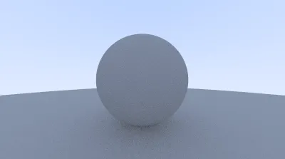
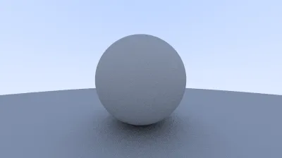
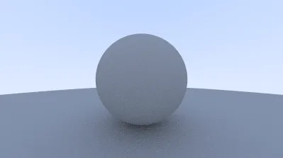
언제나처럼 실행하게 되면, 아래와 처럼 난반사를 하는 Object들이 Image로 잘 나타나는 것을 확인할 수 있다.

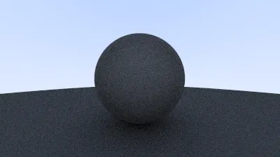
3. Using Gamma Correction for Accurate Color Intensity

우리가 구현한 코드를 보면 ray가 물체에서 난반사 되어 다른 곳을 향하게 되면 50%만 반사 하도록 만들었음에도 굉장히 어두운 결과를 얻게 되었는데 이 때문에 그림자를 넣더라도 확인이 불가능하게 된다. 이 문제를 해결하기 위해서 다른 Image Viewer에서는 보통 Gamma Correction을 이용하여 Object를 조금 더 밝게 수정한다. 우리는 그 중에서도 Gamma 2 로 근사하여 사용할 것이다. Scale된 색상 값을

c

라고 하고 Gamma Correction의 수치를

g

라고 했을 때, 색상 값은

\sqrt[g] c

가 된다.

Gamma 2로 Correction을 수행하게 되면,

\sqrt c

가 된다.

Gamma Correction 수행을 위해 색상 값을 기록하는 color.h의 write_color 함수를 수정하자.

#ifndef COLOR_H
# define COLOR_H

# include "rtweekend.h"
# include <iostream>

void write_color(std::ostream &out, color pixel_color, int samples_per_pixel)
{
	auto r = pixel_color.x();
	auto g = pixel_color.y();
	auto b = pixel_color.z();

	// Divide the color by the number of samples.
	auto scale = 1.0 / samples_per_pixel;
	r = sqrt(scale * r);
	g = sqrt(scale * g);
	b = sqrt(scale * b);

    	// Write the translated [0,255] value of each color component.
    	out << static_cast<int>(255.999 * clamp(r, 0.0, 0.999)) << ' '
        	<< static_cast<int>(255.999 * clamp(g, 0.0, 0.999)) << ' '
        	<< static_cast<int>(255.999 * clamp(b, 0.0, 0.999)) << '\n';
}

#endif
C++
복사

코드를 실행해보면 기존 50% 감소된 빛의 난반사에 Gamma Correction이 적용되어 결정된 색상이 조금 더 밝은 것을 확인할 수 있다.

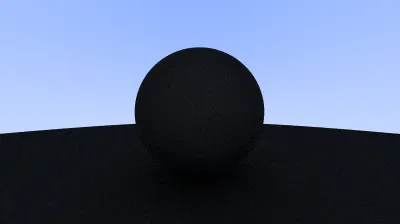
4. Fixing Shadow Acne

Gamma Correction를 통해 실제처럼 만들었다고 해도 여전히 미묘한 버그가 있다. Object에 닿아 반사된 ray는 정확히

t = 0

에 수렴하지 않는다. 따라서

t = -0.00001

혹은

t = 0.00000001

혹은 우리에게 주어지는 구체의 교차 구간에서의 부동 소수점 근사치를 이용하게 된다. 따라서 기존처럼

t

값이 거의

0

에 수렴하는 값은 사용하지 않는다.

t = 0

값 대신에 다른 부동 소수점 값을 사용함에 따라 Shadow Acne 문제를 수정할 수 있다. 아래와 같이 main.cpp를 수정한다.

#include "rtweekend.h"
#include "color.h"
#include "hittable_list.h"
#include "sphere.h"
#include "camera.h"
#include <iostream>

color ray_color(const ray& r, const hittable& world, int depth)
{
	hit_record rec;

	// If we've exceeded the ray bound limit, no more light is gathered.
	if (depth <= 0)
		return (color(0, 0, 0));
	if (world.hit(r, 0.001, infinity, rec))
	{
		point3 target = rec.p + rec.normal + random_in_unit_sphere();
		return (0.5 * ray_color(ray(rec.p, target - rec.p), world, depth - 1));
	}
	vec3 unit_direction = unit_vector(r.direction());
	auto t = 0.5 * (unit_direction.y() + 1.0);
	return (1.0 - t) * color(1.0, 1.0, 1.0) + t * color(0.5, 0.7, 1.0);
}

int main(void)
{
	// Image
	const auto aspect_ratio = 16.0 / 9.0;
	const int image_width = 400;
	const int image_height = static_cast<int>(image_width / aspect_ratio);
	const int samples_per_pixel = 100;
	const int max_depth = 50;

	// World
	hittable_list world;
	world.add(make_shared<sphere>(point3(0, 0, -1), 0.5));
	world.add(make_shared<sphere>(point3(0, -100.5, -1), 100));

	// Camera
	camera cam;

	// Render
	std::cout << "P3\n" << image_width << ' ' << image_height << "\n255\n";

	for (int j = image_height - 1; j >= 0; --j)
	{
		std::cerr << "\rScanlines Remaining: " << j << ' ' << std::flush;
		for (int i = 0; i < image_width; ++i)
		{
			color pixel_color(0, 0, 0);
			for (int s = 0; s < samples_per_pixel; ++s)
			{
				auto u = (i + random_double()) / (image_width - 1);
				auto v = (j + random_double()) / (image_height - 1);
				ray r = cam.get_ray(u, v);
				pixel_color += ray_color(r, world, max_depth);
			}
			write_color(std::cout, pixel_color, samples_per_pixel);
		}
	}

	std::cerr << "\nDone.\n";

	return (0);
}
C++
복사

그저 0.0을 0.001로 수정하여 버그를 고쳤을 뿐인데, 실행 결과는 기존과 꽤나 많이 차이나는 것을 볼 수 있다. (심지어 결과를 얻기까지의 시간도 많이 줄어든다.)

5. True Lambertian Reflection

이번 Chapter에서 소개되는 Rejection 알고리즘은 Object 표면에서의 Normal을 따라 단위 구체 내부의 무작위한 점을 생성한다. 구체의 표면에서 무작위 점까지의 Vector는 낮은 확률로 넓은 각도의 난반사를 보이고, 높은 확률로 Normal과 일치하는 결과를 보인다. Normal과 난반사 Vector의 각도를

\phi

라고 했을 때,

위 무작위 Vector를

cos^3(\phi)

로 Scale 하여 얻은 분포를 이용하면 꽤나 유용하게 이 문제를 해결할 수 있다. 얕은 각으로 설정된 무작위 점을 넓은 영역으로 확장하면서도 최종적으로 결정하는 색상에는 적은 영향을 끼치는 것이 가능하다. 이에 비해

cos(\phi)

의 분포를 갖는 올바른 Lambertian은 높은 확률로 Normal에서 가까운 ray를 충분히 멀리 퍼뜨려준다. 또한 이렇게 얻어진 결과는

cos^3(\phi)

의 분포로 이용했던 것에 비해 더 Uniform한 결과를 얻을수 있기 때문에 우리는

cos^3(\phi)

보다는 Lambertian 분포에 조금 더 관심을 두게 된다. Lambertian은 단위 구체 내부가 아닌 단위 구체 표면 위의 임의의 점을 잡음으로써 달성할 수 있다. 단위 구체 표면 위의 점을 잡는 방법은 단순하다. 이전 처럼 단위 구체 내부의 무작위 점을 잡고 unit_vector 함수를 이용하여 단위 Vector로 만들어주면 된다.

위처럼 복잡하게 설명된 것을 요약하면 다음과 같다. 단위 구체 내부의 임의의 점을 잡았던 기존의 코드를 단위 Vector로 만들어주면 된다는 것이다. 수정된 vec3.h의 코드는 아래와 같다.

#ifndef VEC3_H
# define VEC3_H

# include "rtweekend.h"
# include <cmath>
# include <iostream>

using std::sqrt;

class vec3
{
    public:
        vec3() : e{0,0,0} {}
        vec3(double e0, double e1, double e2) : e{e0, e1, e2} {}

        double x() const { return e[0]; }
        double y() const { return e[1]; }
        double z() const { return e[2]; }

        vec3 operator-() const { return vec3(-e[0], -e[1], -e[2]); }
        double operator[](int i) const { return e[i]; }
        double& operator[](int i) { return e[i]; }

        vec3& operator+=(const vec3 &v)
				{
            e[0] += v.e[0];
            e[1] += v.e[1];
            e[2] += v.e[2];
            return *this;
        }

        vec3& operator*=(const double t)
				{
            e[0] *= t;
            e[1] *= t;
            e[2] *= t;
            return *this;
        }

        vec3& operator/=(const double t)
				{
            return *this *= 1/t;
        }

        double length() const
				{
            return sqrt(length_squared());
        }

        double length_squared() const
				{
            return e[0]*e[0] + e[1]*e[1] + e[2]*e[2];
        }

				inline static vec3 random()
				{
					return (vec3(random_double(), random_double(), random_double()));
				}

				inline static vec3 random(double min, double max)
				{
					return (vec3(random_double(min, max), random_double(min, max), random_double(min, max)));
				}


    public:
        double e[3];
};

// Type aliases for vec3
using point3 = vec3;   // 3D point
using color = vec3;    // RGB color

// vec3 Utility Functions
inline std::ostream& operator<<(std::ostream &out, const vec3 &v)
{
    return out << v.e[0] << ' ' << v.e[1] << ' ' << v.e[2];
}

inline vec3 operator+(const vec3 &u, const vec3 &v)
{
    return vec3(u.e[0] + v.e[0], u.e[1] + v.e[1], u.e[2] + v.e[2]);
}

inline vec3 operator-(const vec3 &u, const vec3 &v)
{
    return vec3(u.e[0] - v.e[0], u.e[1] - v.e[1], u.e[2] - v.e[2]);
}

inline vec3 operator*(const vec3 &u, const vec3 &v)
{
    return vec3(u.e[0] * v.e[0], u.e[1] * v.e[1], u.e[2] * v.e[2]);
}

inline vec3 operator*(double t, const vec3 &v)
{
    return vec3(t*v.e[0], t*v.e[1], t*v.e[2]);
}

inline vec3 operator*(const vec3 &v, double t)
{
    return t * v;
}

inline vec3 operator/(vec3 v, double t)
{
    return (1/t) * v;
}

inline double dot(const vec3 &u, const vec3 &v)
{
    return u.e[0] * v.e[0]
         + u.e[1] * v.e[1]
         + u.e[2] * v.e[2];
}

inline vec3 cross(const vec3 &u, const vec3 &v)
{
    return vec3(u.e[1] * v.e[2] - u.e[2] * v.e[1],
                u.e[2] * v.e[0] - u.e[0] * v.e[2],
                u.e[0] * v.e[1] - u.e[1] * v.e[0]);
}

inline vec3 unit_vector(vec3 v)
{
    return v / v.length();
}

inline vec3 random_in_unit_sphere()
{
	while (true)
	{
		auto p = vec3::random(-1, 1);
		if (p.length_squared() >= 1)
			continue;
		return (p);
	}
}

vec3 random_unit_vector()
{
	return (unit_vector(random_in_unit_sphere()));
}

#endif
C++
복사

위 코드로 고치면 아래 사진과 같이 무작위로 잡힌 점이 곧 단위 Vector로 변환되어 사용할 수 있게 된다.

따라서 기존에 random_in_unit_sphere를 이용하던 main.cpp도 random_unit_vector를 호출하도록 변경해준다.

#include "rtweekend.h"
#include "color.h"
#include "hittable_list.h"
#include "sphere.h"
#include "camera.h"
#include <iostream>

color ray_color(const ray& r, const hittable& world, int depth)
{
	hit_record rec;

	// If we've exceeded the ray bound limit, no more light is gathered.
	if (depth <= 0)
		return (color(0, 0, 0));
	if (world.hit(r, 0.001, infinity, rec))
	{
		point3 target = rec.p + rec.normal + random_unit_vector();
		return (0.5 * ray_color(ray(rec.p, target - rec.p), world, depth - 1));
	}
	vec3 unit_direction = unit_vector(r.direction());
	auto t = 0.5 * (unit_direction.y() + 1.0);
	return (1.0 - t) * color(1.0, 1.0, 1.0) + t * color(0.5, 0.7, 1.0);
}

int main(void)
{
	// Image
	const auto aspect_ratio = 16.0 / 9.0;
	const int image_width = 400;
	const int image_height = static_cast<int>(image_width / aspect_ratio);
	const int samples_per_pixel = 100;
	const int max_depth = 50;

	// World
	hittable_list world;
	world.add(make_shared<sphere>(point3(0, 0, -1), 0.5));
	world.add(make_shared<sphere>(point3(0, -100.5, -1), 100));

	// Camera
	camera cam;

	// Render
	std::cout << "P3\n" << image_width << ' ' << image_height << "\n255\n";

	for (int j = image_height - 1; j >= 0; --j)
	{
		std::cerr << "\rScanlines Remaining: " << j << ' ' << std::flush;
		for (int i = 0; i < image_width; ++i)
		{
			color pixel_color(0, 0, 0);
			for (int s = 0; s < samples_per_pixel; ++s)
			{
				auto u = (i + random_double()) / (image_width - 1);
				auto v = (j + random_double()) / (image_height - 1);
				ray r = cam.get_ray(u, v);
				pixel_color += ray_color(r, world, max_depth);
			}
			write_color(std::cout, pixel_color, samples_per_pixel);
		}
	}

	std::cerr << "\nDone.\n";

	return (0);
}
C++
복사

Lambertian을 적용한 Image를 보면 Gamma Correction을 적용했던 것보다도 상당히 밝아진 구체를 확인할 수 있다. 이는 실제 Object처럼 빛의 난반사가 Normal을 향하지 않고 골고루 퍼졌다는 것을 암시한다.

Gamma Correction과 Lambertian의 적용이 굉장히 쉬운 것에 반해 두 방법을 적용한 Image와 두 방법을 적용하지 않은 (Chapter 7까지의 결과) Image의 시각적 차이를 인지하는 것은 굉장히 중요하다.

Chapter 8까지의 결과를 보면 그림자가 조금은 덜 뚜렷해진다.

Chapter 8까지의 결과를 보면 구체의 외관이 더 밝아진다.

위 2가지 사항들은 난반사된 ray가 Uniform한 확률 분포로 흩어짐과 동시에 구체의 Normal과 덜 일치하도록 흩어졌기 때문이다. 이는 곧 Camera를 향해 반사된 ray가 기존보다 더 많이 들어오기 때문에 밝아보이는 것이다. 또한 그림자의 경우, 기존보다 ray가 적은 횟수로 반사를 만들어 내기 때문에 큰 구체 위의 작은 구체가 이루는 그림자가 조금은 더 밝아지면서 덜 뚜렷해지는 것이다.

6. An Alternative Diffuse Formulation

위에서 제시된 Lambertian 분포는 부정확한 근사치가 입증되기 전까지 꽤 오랜 기간동안 이용되어 왔다. 수학적으로 분포의 부정확함을 증명하는 것이 어려웠고,

cos(\phi)

의 분포가 왜 바람직한지 이해하는 것이 상당히 직관적이었기 때문에 지속되어 온 것이다. 일상의 Object들은 완벽하게 난반사를 이루고 있기에 Object가 빛에 대해서 어떻게 작용하는지에 대한 우리의 시각적 직관이 형편 없이 형성되는 것은 흔하지 않은 일이다.

학습을 위해서 강의에서는 꽤 이해하기 쉬운 난반사를 이용했었다. 위에서 소개한 Rejection과 Lambertian인데, 이 두 방법은 ray가 Object에 닿은 점의 Normal을 통해 얻어낸 Random Vector를 기반으로 한다. 두 방법의 차이는 Vector의 길이가 Random으로 하는지 단위 길이로 하는지이다. 이 때 후자에 대해서 Lambertian의 방식을 이용할 때, 왜 Random Vector가 Normal과 달라야하는지 바로 이해하는 것이 어려울 수 있다. 따라서 조금 더 직관적인 방법은 Normal에 의존하지 않고 ray가 닿은 지점을 기준으로 모든 각도로 퍼지는 ray를 Uniform한 확률 분포를 갖도록 만드는 것이다. 초기의 많은 RT 논문들은 Lambertian이 채택되기 전에는 Normal에 의존하지 않은 난반사를 이용했었다. 이 방법을 Hemisphere Scattering이라고 한다.

따라서 기존의 Lambertian을 따를 때 작성했던 random_in_unit_sphere를 이용하여 random_in_hemisphere 함수를 작성하고, 무작위 점을 Normal에 연산하여 구한 Vector를 random_in_hemisphere 함수의 반환 값으로 대치한다. vec3.h에 해당 함수를 추가하고, 호출하는 main.cpp를 고쳐보자. 코드는 아래와 같다.

기존의 Lambertian에서는 ray가 닿은 점

P

+ Normal + 무작위 점

S

로 Random Vector를 이용했다면, Hemisphere Scattering에서는 Normal에 대한 의존을 없애 ray가 닿은 점

P

+ random_in_hemisphere의 반환 Vector로 변경한 것이다.

#ifndef VEC3_H
# define VEC3_H

# include "rtweekend.h"
# include <cmath>
# include <iostream>

using std::sqrt;

class vec3
{
    public:
        vec3() : e{0,0,0} {}
        vec3(double e0, double e1, double e2) : e{e0, e1, e2} {}

        double x() const { return e[0]; }
        double y() const { return e[1]; }
        double z() const { return e[2]; }

        vec3 operator-() const { return vec3(-e[0], -e[1], -e[2]); }
        double operator[](int i) const { return e[i]; }
        double& operator[](int i) { return e[i]; }

        vec3& operator+=(const vec3 &v)
	{
            e[0] += v.e[0];
            e[1] += v.e[1];
            e[2] += v.e[2];
            return *this;
        }

        vec3& operator*=(const double t)
	{
            e[0] *= t;
            e[1] *= t;
            e[2] *= t;
            return *this;
        }

        vec3& operator/=(const double t)
	{
            return *this *= 1/t;
        }

        double length() const
	{
            return sqrt(length_squared());
        }

        double length_squared() const
	{
            return e[0]*e[0] + e[1]*e[1] + e[2]*e[2];
        }

	inline static vec3 random()
	{
		return (vec3(random_double(), random_double(), random_double()));
	}

	inline static vec3 random(double min, double max)
	{
		return (vec3(random_double(min, max), random_double(min, max), random_double(min, max)));
	}


    public:
        double e[3];
};

// Type aliases for vec3
using point3 = vec3;   // 3D point
using color = vec3;    // RGB color

// vec3 Utility Functions
inline std::ostream& operator<<(std::ostream &out, const vec3 &v)
{
    return out << v.e[0] << ' ' << v.e[1] << ' ' << v.e[2];
}

inline vec3 operator+(const vec3 &u, const vec3 &v)
{
    return vec3(u.e[0] + v.e[0], u.e[1] + v.e[1], u.e[2] + v.e[2]);
}

inline vec3 operator-(const vec3 &u, const vec3 &v)
{
    return vec3(u.e[0] - v.e[0], u.e[1] - v.e[1], u.e[2] - v.e[2]);
}

inline vec3 operator*(const vec3 &u, const vec3 &v)
{
    return vec3(u.e[0] * v.e[0], u.e[1] * v.e[1], u.e[2] * v.e[2]);
}

inline vec3 operator*(double t, const vec3 &v)
{
    return vec3(t*v.e[0], t*v.e[1], t*v.e[2]);
}

inline vec3 operator*(const vec3 &v, double t)
{
    return t * v;
}

inline vec3 operator/(vec3 v, double t)
{
    return (1/t) * v;
}

inline double dot(const vec3 &u, const vec3 &v)
{
    return u.e[0] * v.e[0]
         + u.e[1] * v.e[1]
         + u.e[2] * v.e[2];
}

inline vec3 cross(const vec3 &u, const vec3 &v)
{
    return vec3(u.e[1] * v.e[2] - u.e[2] * v.e[1],
                u.e[2] * v.e[0] - u.e[0] * v.e[2],
                u.e[0] * v.e[1] - u.e[1] * v.e[0]);
}

inline vec3 unit_vector(vec3 v)
{
    return v / v.length();
}

inline vec3 random_in_unit_sphere()
{
	while (true)
	{
		auto p = vec3::random(-1, 1);
		if (p.length_squared() >= 1)
			continue;
		return (p);
	}
}

vec3 random_unit_vector()
{
	return (unit_vector(random_in_unit_sphere()));
}

vec3 random_in_hemisphere(const vec3& normal)
{
	vec3 in_unit_sphere = random_in_unit_sphere();
	if (dot(in_unit_sphere, normal) > 0.0) // In the same hemisphere as the normal
		return (in_unit_sphere);
	return (-in_unit_sphere);
}

#endif
C++
복사

#include "rtweekend.h"
#include "color.h"
#include "hittable_list.h"
#include "sphere.h"
#include "camera.h"
#include "vec3.h"
#include <iostream>

color ray_color(const ray& r, const hittable& world, int depth)
{
	hit_record rec;

	// If we've exceeded the ray bound limit, no more light is gathered.
	if (depth <= 0)
		return (color(0, 0, 0));
	if (world.hit(r, 0.001, infinity, rec))
	{
		point3 target = rec.p + random_in_hemisphere(rec.normal);
		return (0.5 * ray_color(ray(rec.p, target - rec.p), world, depth - 1));
	}
	vec3 unit_direction = unit_vector(r.direction());
	auto t = 0.5 * (unit_direction.y() + 1.0);
	return (1.0 - t) * color(1.0, 1.0, 1.0) + t * color(0.5, 0.7, 1.0);
}

int main(void)
{
	// Image
	const auto aspect_ratio = 16.0 / 9.0;
	const int image_width = 400;
	const int image_height = static_cast<int>(image_width / aspect_ratio);
	const int samples_per_pixel = 100;
	const int max_depth = 50;

	// World
	hittable_list world;
	world.add(make_shared<sphere>(point3(0, 0, -1), 0.5));
	world.add(make_shared<sphere>(point3(0, -100.5, -1), 100));

	// Camera
	camera cam;

	// Render
	std::cout << "P3\n" << image_width << ' ' << image_height << "\n255\n";

	for (int j = image_height - 1; j >= 0; --j)
	{
		std::cerr << "\rScanlines Remaining: " << j << ' ' << std::flush;
		for (int i = 0; i < image_width; ++i)
		{
			color pixel_color(0, 0, 0);
			for (int s = 0; s < samples_per_pixel; ++s)
			{
				auto u = (i + random_double()) / (image_width - 1);
				auto v = (j + random_double()) / (image_height - 1);
				ray r = cam.get_ray(u, v);
				pixel_color += ray_color(r, world, max_depth);
			}
			write_color(std::cout, pixel_color, samples_per_pixel);
		}
	}

	std::cerr << "\nDone.\n";

	return (0);
}
C++
복사

코드를 실행해보면 아래와 같은 Image를 얻을 수 있는데 이는 Lambertian의 결과와 상당히 비슷한 것을 보아 나쁘지 않은 성능을 예상할 수 있다. Chapter가 진행될수록 world에는 더욱 더 많은 Object들이 들어가면서 Screen이 복잡해지게 된다. 따라서 여기에 제시된 Hemisphere Scattering을 이용한 난반사를 적용하는 것을 권장한다. 많은 Screen의 중점은 난반사를 내는 Object들의 불균형이다. 다양한 방법으로 Screen에 난반사를 구현해보다 보면 각 방법들이 어떤 영향을 끼치는지에 대한 통찰력을 얻을 수 있을 것이다.